Walking Biped Robot
We used a single model-predictive controller to make a simulated biped stand, walk, run 10 meters, and climb stairs.
Ardalan Aryashad, Dakota Mercer, Ibrahim K. Ozaslan
AME 556: Robot Dynamics and Control · Fall 2024 · USC
By the last week of the semester we had a two-legged robot that could stand up, squat, walk forward and backward, and run 10 meters in 9.08 seconds — all of it driven by a single optimization that re-solves itself every 40 milliseconds and decides, from scratch, how hard each foot should push on the ground. This page is the story of that robot, the one stair-climbing task that nearly broke us, the obstacle course we ran out of time to finish, and the sixteen weeks of homework that quietly made the whole thing possible.
It’s the project that turned AME 556 from “a controls class” into the reason I think about robots the way I do now.
Sixteen weeks of homework, hiding a robot
The thing nobody tells you about the final project is that you’ve been building it since week one. Each homework set was a single piece of the controller, handed to us out of order, and the project was where they finally clicked into one machine.
The semester, read as one long build-up. HW4 — LQR and an MPC written as a quadratic program solved with quadprog — is the piece the project leans on most directly; the report literally says "since it is similar to our homework, we skip the details."
HW1 was pure geometry — rotating triangles in MATLAB, stacking rotation matrices, chaining homogeneous transforms to find where the end of a limb lands. It felt abstract at the time. In the project, that’s the exact math (rot2D(theta)·rot2D(q1)·…) that locates each foot in the world so the controller knows where contact is.
HW2 was where things started moving: writing equations of motion by hand and integrating them with ode45 — a ball with drag, an inverted pendulum, a UAV. This is the habit of modeling first that the whole project rests on.
HW3 introduced the linear inverted pendulum model and dropped us into MATLAB Simscape with real contact and gravity — the same simulation environment the biped lives in. The inverted pendulum, it turns out, is the entire intuition for balancing a walking robot: keep the center of mass over a moving support point.
HW4 is the one that mattered most. We built an LQR controller, then re-derived an MPC as a quadratic program — stacking the prediction horizon into big block matrices with Kronecker products and handing it to quadprog under state and input constraints. That code is, almost verbatim, the brain of the biped.
HW5 went nonlinear — input–output (feedback) linearization and a CLF-QP controller — which is the language for reasoning about why a constrained controller stays stable when the dynamics aren’t linear at all.
Five homeworks, one robot. Seeing that arc only in hindsight is one of my favorite things about the class.
One controller runs the whole robot
The robot itself is deliberately simple: a 2D body with two legs, each leg a hip and a knee (joints $q_1,q_2$ on the left, $q_3,q_4$ on the right), point feet, built in Simscape so that gravity, ground contact, and friction are all real physics rather than something we hand-wave.
What I find genuinely elegant is that every task on this page runs the same controller. We never wrote a “walk” mode and a “run” mode and a “stairs” mode. We wrote one optimization-based controller and changed its desired trajectory and gait schedule — that’s it.
The control architecture. The gait schedule decides, at each instant, which leg is on the ground (stance) and which is in the air (swing). Stance legs get their ground-reaction forces from the MPC; swing legs get a force from a PD law that steers the foot to its next landing spot. A Jacobian transpose turns both into joint torques. Changing the desired trajectory and the gait timing is the only thing that separates "walk" from "run" from "climb."
The MPC plans over a short horizon on a single-rigid-body model of the body — position $x$, height $y$, pitch $\theta$, their velocities, plus a gravity term — and treats the foot ground-reaction forces as the decision variables. Every cycle it solves a quadratic program (the HW4 machinery) for the forces that best track the desired body motion, subject to honest constraints: forces can only push, never pull, and they have to stay inside the friction cone (we used a 0.7 friction coefficient) and under a 250 N cap. We weighted the cost heavily toward keeping height and pitch ($Q$ on $y$ and $\theta$ at 5000 and 3000) because a biped that loses its pitch falls over instantly.
The leg that’s off the ground doesn’t get a force from the MPC — it gets steered by a small PD controller to a target foot position computed from a capture-point–style law (step out in the direction you’re already moving, by half a step’s worth, and correct toward the desired speed). That single split — stance handled by optimization, swing handled by PD — is the whole trick.
Teaching it to walk
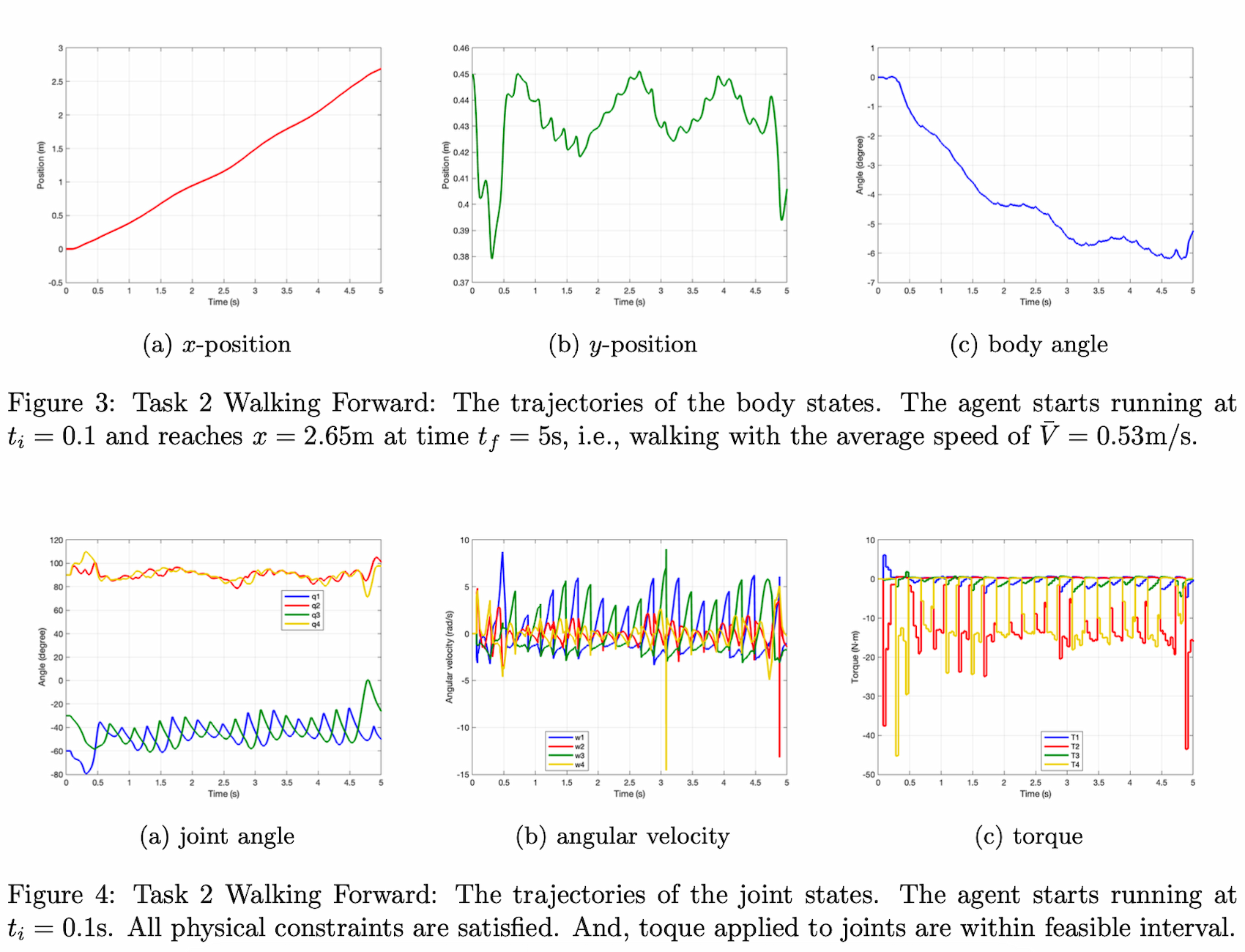
Standing came first: hold the body at 0.45 m, then command the height up to 0.5 m and back down to 0.4 m and back, and watch the MPC squat on command without tipping. Once it could balance, walking was “just” adding the gait schedule — alternating five control steps of stance with five of swing per leg — and giving the body a forward velocity target.
Walking forward — desired foot speed 1 m/s, body speed 0.6 m/s, covering 2.65 m in 5 s.
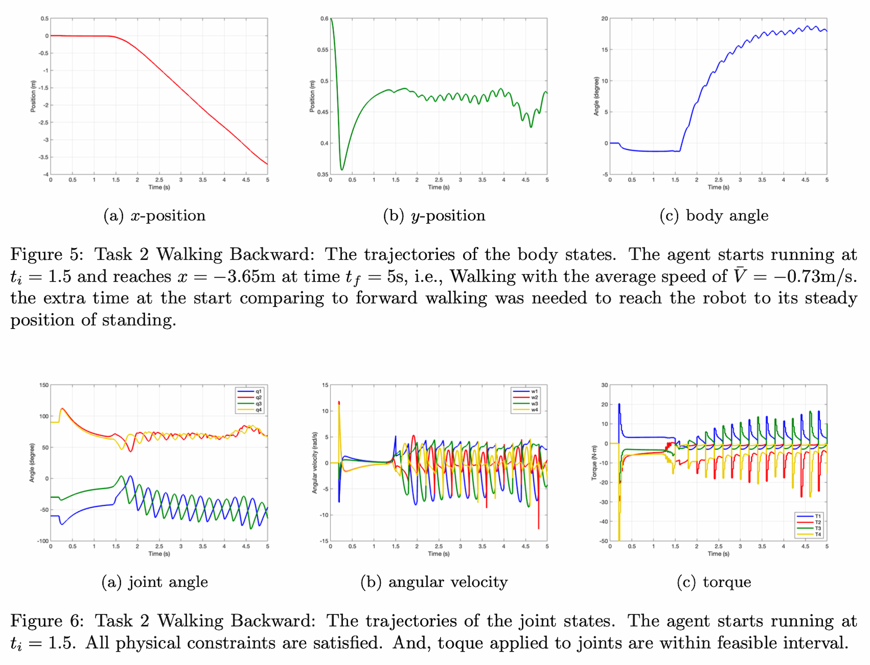
Walking backward — the same controller, a negative velocity target, and a longer settle before the first step.
Backward walking taught us a small but stubborn lesson: it needed more time standing still before it could start. The robot had to fully settle into a stable stance before reversing, otherwise the first backward step would catch it mid-wobble and throw the pitch off. That extra second and a half of “do nothing” at the start was the difference between a clean −0.73 m/s gait and a faceplant.
Running: where the score is just speed
Task 3 was scored on a stopwatch: cover 10 meters, and your points are 200 divided by your time. No partial credit for elegance — faster is the whole grade. That changes how you tune. Suddenly the question isn’t “is it stable” but “how aggressively can I push the body velocity before stability gives out.”
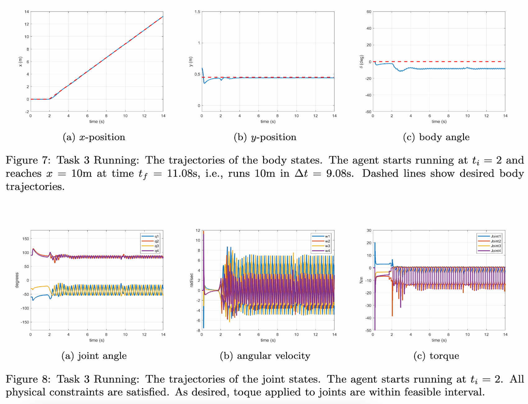
The running gait pushes the body target to 1.1 m/s with a 1 m/s foot swing and a 6 cm step height.
We pushed the desired body velocity to 1.1 m/s, kept the foot swinging at 1 m/s with a 6 cm clearance, and retuned the swing-leg PD gains until it would commit to the speed without the pitch running away. The robot ran the 10 meters in 9.08 seconds — good for 22 points, our highest-scoring task. Getting there was almost entirely gain-tuning: nudge a swing gain, watch the torque plot spike into its limit, back it off, try again.
Stairs, where everything we’d tuned fell apart
This is the task I learned the most from, because it’s the one where our nice clean approach stopped working and we had to get our hands dirty.
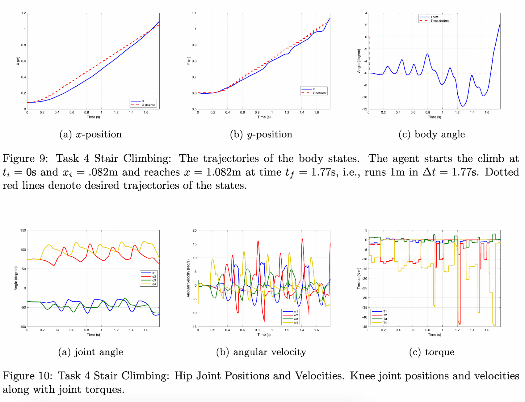
Climbing five stairs in 1.79 s. Getting the feet to clear each step instead of stubbing into its edge was the entire battle.
On flat ground, gait scheduling is forgiving — the floor is always at the same height, so a foot coming down lands where you expect. On stairs, the ground keeps jumping up by a step, and the timing that worked perfectly on flat ground would slam a foot straight into the riser of the next step. A few things we had to discover the hard way:
- The 40 ms MPC clock was too slow for the legs. The PD swing controller, running at the same 40 ms as the MPC, lagged badly enough that the foot would already be colliding with a stair before the controller reacted. We split the rates — PD swing at 10 ms, MPC still at 40 ms — and the foot finally tracked its target in time.
- A sine-wave foot path doesn’t clear a stair; a square wave does. The smooth sinusoidal swing arc we used for walking would clip the corner of the step. Switching the desired vertical foot motion to a square wave — snap up, hold high, snap down — gave the clearance to get over each riser.
- We tried throwing away the gait schedule entirely. One experiment replaced timed stepping with torque/contact sensing: AND/OR-gate logic in Simulink that detected when a foot actually touched a stair, so we wouldn’t have to hand-time the steps. It removed the painful timing problem — but it created a worse one. Contact detection was now out of sync with the MPC, so a foot would land and then wait up to 40 ms for the next MPC solve before getting any force, and in that gap it would slip. We went back to gait scheduling.
- The two legs needed different gains. One leg consistently lagged the other, building up more tracking error, which kept tripping the speed and torque limits. We ended up tuning the left and right legs separately — slightly higher derivative gains on the lagging leg — which is exactly the kind of asymmetric, un-pretty fix you only find by staring at why one specific foot keeps violating a constraint.
The payoff: five stairs in 1.79 seconds. Less elegant than the flat-ground gaits, but it’s the task where I actually understood why the textbook controller wasn’t enough and what it takes to bridge from a clean model to messy contact.
The task we didn’t finish
I want to be honest about Task 5, the obstacle course, because the report says it plainly: “could not complete the task, but made progress.” We ran out of semester.
The course needed jumping, and a jump is a genuinely different beast from a step. A walking gait always has one foot down; a jump needs both feet to push together, then a flight phase where neither foot touches anything, then a two-foot landing — a gait cycle like [1 1 1 0 0 0 0 0 1 1] for both legs at once instead of the alternating pattern that does everything else. We worked out the flight-phase foot-placement law (keep each foot trailing the center of mass at a fixed offset so it’s positioned to catch the landing) and the gait structure, but we didn’t get a reliable jump-land-continue working before the deadline.
It cost us the points — our total landed at 73 — and I’d rather show that than pretend the project was a clean sweep. Knowing exactly where it broke (the transition into and out of flight, where the MPC briefly has no contact forces to command at all) is its own kind of result.
What the course actually taught me
The honest takeaway isn’t any single controller. It’s that I came into AME 556 thinking control was a bag of formulas and left thinking of it as one continuous skill: model the thing, decide what you want it to do, and pose that as an optimization the computer can solve fast enough to keep up with reality.
Three things stuck with me hardest:
- A model is a choice, and the right model is small. The MPC doesn’t reason about the legs at all — it pretends the robot is one rigid body and lets the legs be force vectors. That deliberate simplification is what makes the QP small enough to solve every 40 ms. Knowing what to ignore turned out to be more important than modeling everything.
- Constraints are where the physics actually lives. The friction cone, the no-pull-on-the-ground rule, the torque saturations — those inequalities are the difference between a robot and a video game. Most of the real work was making sure the optimizer respected them.
- Tuning is not a footnote. Every task on this page came down to days of nudging gains while watching a torque plot kiss its limit. The theory gets you a controller that can work; the patience gets you one that does.
I’d point to this project from my coursework as the start of robotic ambition, because it’s the one where the math from week one and the gains I tweaked at 2 a.m. in finals week ended up being the same conversation.